Text to image에 조건을 부여하기 위해 사용하는 ControlNet 의 논문을 읽고 내용을 간략하게 정리해보았다.
Abstract
- ControlNet : pre-trained text-to-image에 공간적인 조건을 주는 아키텍쳐
- encoding layers만 많은 이미지로 재학습 한다.
- zero convolution으로 연결
→ 0으로 초기화 되어서 점점 커지며 불필요한 노이즈가 파인튜닝에 영향을 못미치도록 함.
1. Introduction
- text-to-image를 공간적 요소에 대한 control에 한계가 있음.
- text를 통해 설명이 어렵기 때문
- 추가적인 이미지로 공간적인 컨트롤이 가능하다.
- image-to-image 모델은 conditioning 이미지에서 target 이미지로의 매핑을 배울 수 있다.
- spatial mask, image editing instruction 등으로 text-to-image 모델을 control하려는 시도가 있었음
→ 어떤 문제들은 denoising process에 제한을 주는 등으로 풀릴 수 있겠지만 end-to-end learning과 data driven solution이 필요함. - specific condition 학습을 위한 데이터 부족 문제가 있음
→ 이 데이터로 large pre-trained model을 파인튜닝 이슈가 발생할 것이다. - ControlNet
- end-to-end로 large pretrained text-to-image의 continional control을 학습하는 아키텍쳐
- large model의 파라미터를 locking하고 encoding layer에서 trainable copy를 만들어 모델의 능력과 질을 보존한다.
- large train model을 다양한 conditional control을 학습하기 위한 backbone으로 취급
- trainable copy와 원래의 locked model은 'zero convolution' layer로 연결됨
- Summary
- ControlNet 제안
- StableDiffusion을 Canny edge, segmentation map 등으로 condition 줄 수 있는 ControlNet 발표
- Vailidate method
2. Related Works
2.1. Finetuning Neural Networks
- 원래 네트워크의 그냥 데이터를 추가해서 학습을 이어가는 파인튜닝 기법도 있지만, overfitting, mode collapse, catastrophic forgetting 등의 문제를 야기함.
- HyperNetwork : 큰 모델의 weight에 영향을 미치는 작은 RNN을 학습
→ GAN이나 stable diffusion에 적용되어 style trasfer 등에 사용 - Apapter : NLP에서 새로운 modul layer를 transformer에 임베딩해 다른 task에 커스터마이징.
- Computer vison에서는 CLIP과 함께 사용되어 backbone 모델을 다른 task로 전환시킴
- T2I-Adapter라는 Stable Diffusion에 추가적인 컨디션을 위해 사용된 어댑터도 있음.
- Additive Learning : 원래 모델 weight을 freeze하고, 작은 수의 새로운 파라미터를 더함.
- LoRA : low-rank matrices로 파라미터들의 offset을 학습
- Zero-Initialized Layers : Neural Net의 파라미터를 0으로 초기화 하는 연구
2.2. Image Diffusion
- Image Diffusion Model
- LDM → Latent Space에서 diffusion step을 수행해서 계산량 낮춤
- Text-to-Image → CLIP으로 text input을 latent로 보냄
- Glide, Disco Diffusion, Stable Diffusion, ...,
- Controlling Image Diffusion Model
- Text-guided control → 프롬프트를 조정하는 것 , CLIP feature 다루기, cross-attention을 수정하는 것에 초점을 맞춤
- SpaText : segmentation mask를 localized token embedding에 매핑
- GLIGEN : attention layer의 새 파라미터 학습
- Textual Inversion & Dream Booth : 작은 데이터셋으로 학습해서 개인화된 콘텐츠 생성
- Prompt-based image editing
2.3. Image-to-Image Translation
- Conditional GANs and transformer는 다른 이미지 도메인들 사이의 매핑을 학습할 수 있다.
3. Method

3.1. ControlNet
- additional condition을 neural network에 주입한다.
- network block : 함께 쓰여 작은 층을 형성하는 여러 층들의 집합(resnet block, multi-head attention block 등)

- Neural network block $F(\cdot; \Theta)$의 연산:
$$ y = F(x; \Theta) $$
where $x, y \in \mathbb{R}^{h\times w \times c}$ - ControlNet은 pretrained neural block에 추가되어, 원래 블럭의 파라미터 $\Theta$를 freeze하고 trainable copy $\Theta_c$를 생성
- Trainable copy는 condition vector $c$를 추가 입력받음
- Zero convolution $Z(\cdot; \cdot)$으로 연결:
$$
y_c = F(x; \Theta) + Z(F(x + Z(c; \Theta_{z1}); \Theta_c); \Theta_{z2})
$$ - 첫 training step에서 $Z(\cdot; \Theta_{z1})$과 $Z(\cdot; \Theta_{z2})$는 0으로 초기화 → $y_c = y$
3.2. ControlNet for Text-to-Image Diffusion

- ControlNet은 UNet의 각 encoder 블럭에 적용
- Stable Diffusion의 경우 input conditioning image를 latent space로 변환:
$$ c_f = \mathcal{C}(c) $$
where $\mathcal{C}(\cdot)$는 4-layer convolutional network
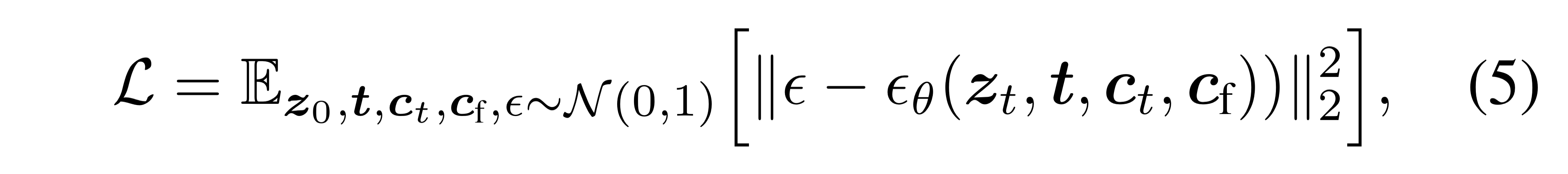
3.3. Training

- Objective function:
$$
\mathcal{L} = \mathbb{E}_{z_0, t, c_t, c_f, \epsilon \sim \mathcal{N}(0,1)} \left[ |\epsilon - \epsilon_\theta(z_t, t, c_t, c_f) |_2^2 \right]
$$ - Sudden convergence phenomenon 관찰
3.4. Inference

- Classifier-free guidance resolution weighting:
$$
\epsilon_{prd} = \epsilon_{uc} + \beta_{cfg}(\epsilon_c - \epsilon_{uc})
$$ - 각 resolution level $i$에서 가중치 적용:
$$
\hat{\epsilon}\theta^{(i)} = w_i \cdot \epsilon{prd}^{(i)} + (1 - w_i) \cdot \epsilon_c^{(i)}
$$
4. Experiment
4.1. Qualitative Result

4.2. Ablative Study


4.3. Quantitative Evaluation


- FID Score:
$$
\text{FID} = |\mu_r - \mu_g|^2 + \text{Tr}(\Sigma_r + \Sigma_g - 2(\Sigma_r \Sigma_g)^{1/2})
$$ - CLIP Score:
$$
\text{CLIP Score} = \frac{1}{N} \sum_{i=1}^N \text{cosine}(E_t(p_i), E_i(x_i))
$$
4.4. Comparison to Previous Method


'데이터 > Machine Learning' 카테고리의 다른 글
| FRIEREN: Efficient Video-to-Audio Generation Network with Rectified Flow Matching (0) | 2025.02.02 |
|---|---|
| Adding Conditional Control to Text-to-Image Diffusion Models 논문 리뷰 (0) | 2025.01.05 |
| [논문 정리]Introduction to VLM(3/3) (1) | 2024.11.24 |
| [논문 정리]Introduction to VLM(2/3) (0) | 2024.11.10 |
| [논문 정리]Introduction to VLM(1/3) (2) | 2024.10.27 |


